Question
Statistics are used to compare and sometimes identify authors. The following lists shows a simple random sample that compares the letter counts for three authors.
Terry: 7; 9; 3; 3; 3; 4; 1; 3; 2; 2 Davis: 3; 3; 3; 4; 1; 4; 3; 2; 3; 1 Maris: 2; 3; 4; 4; 4; 6; 6; 6; 8; 3
a. Make a dot plot for the three authors and compare the shapes.
b. Calculate the mean for each.
c. Calculate the median for each.
d. Describe any pattern you notice between the shape and the measures of center.
a. Dot plots and distribution shapes
Each dot in the figure is one of the ten supplied observations. The common horizontal scale makes the tails comparable.
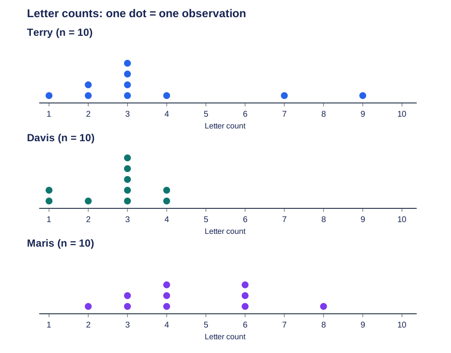
The frequencies below make every plotted point independently checkable:
| Letter count | Terry | Davis | Maris |
|---|---|---|---|
| 1 | 1 | 2 | 0 |
| 2 | 2 | 1 | 1 |
| 3 | 4 | 5 | 2 |
| 4 | 1 | 2 | 3 |
| 5 | 0 | 0 | 0 |
| 6 | 0 | 0 | 3 |
| 7 | 1 | 0 | 0 |
| 8 | 0 | 0 | 1 |
| 9 | 1 | 0 | 0 |
| 10 | 0 | 0 | 0 |
| Total | 10 | 10 | 10 |
Terry has a positive (right) skew: most observations are near 2–4, with isolated high values at 7 and 9. Davis has a negative (left) skew: the peak is at 3 and the tail extends farther toward 1 than toward 4.
Maris is an irregular, bimodal sample, not exactly symmetric. Its two modes are 4 and 6. For symmetry around their midpoint 5, the frequencies at 3 and 7 would need to match, but they are 2 and 0. The rightmost observation is 8 and the leftmost is 2; equal endpoints alone do not establish symmetry. Avoid forcing this small sample into a perfectly symmetric model.
b. Means
c. Medians
With ten observations, average the fifth and sixth values after sorting.
| Author | Sorted observations | Fifth and sixth | Median |
|---|---|---|---|
| Terry | 1, 2, 2, 3, 3, 3, 3, 4, 7, 9 | 3 and 3 | 3 |
| Davis | 1, 1, 2, 3, 3, 3, 3, 3, 4, 4 | 3 and 3 | 3 |
| Maris | 2, 3, 3, 4, 4, 4, 6, 6, 6, 8 | 4 and 4 | 4 |
d. Pattern between shape and center
For Terry, : high values pull the mean into the right tail. For Davis, : low values pull the mean toward the left tail. These illustrate the usual relationship between tail direction and mean versus median.
Maris has mean 4.6 and median 4, but the unequal frequencies and two modes require a separate shape description. The source's worked solution labels it symmetric; the supplied numbers do not support exact symmetry. Likewise, mean–median ordering is a useful clue, not a universal rule for all discrete or multimodal distributions. The data alone do not identify an author beyond these labeled samples.
Original exercise attribution
Adapted in layout from Barbara Illowsky and Susan Dean, Introductory Statistics (OpenStax College, 2013), CC BY 4.0. Download for free at http://cnx.org/content/col11562/latest/. The exercise data and all subquestions are retained; the worked explanation and plotted dots are provided here.
Evidence boundary
This answer uses all three data lists and all four parts of Example 2.31 in the 2013 OpenStax PDF. The dot plots are reconstructed from the exact supplied observations. Maris is not exactly symmetric despite the source solution’s description; no data are changed to fit that claim. Mean–median ordering is not treated as a universal skewness test.
Sources
Эти источники подтверждают изложенные выше концепции и методы.